
In dynamic and control systems one of the most common elements is a lag. This is a first order slowing or delay of an action. It is generally modeled by a transfer from a constant potential to a storage element through a resistance. The key characteristic is that the rate of flow is proportional to the difference in potential between the source and the storage element. In electronics it is commonly charging a capacitor through a resistor from a constant voltage source. Other examples include: adding air to a tire from a constant pressure source, filling a water tank from the bottom using a constant pressure source, certain chemical reactions to equilibrium, spinning up a flywheel from a constant RPM drive through a fluid coupler, heat transfer by conduction from a constant temperature source to an object at a different temperature, or damped spring compression with a constant force. The response of these systems to a step change in potential looks like this:
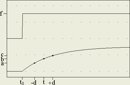
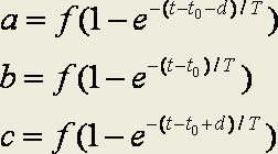
Mathematically this response is the exponential shown below where b is the instantaneous value, f is the final value, t0 is the step time, T is the lag time constant, and t is the time variable. If you want to predict the future final value in a control system to speed up loop response time you have to sample three points and then solve these three equations to find f in real time. In the normal scheme of things this will involve calculating logarithms (inverse exponentials) which will take a lot of CPU time, time you may not have for a high speed control system. Here’s a surprising shortcut. If the three samples are at an equal time interval, typical of sampled data systems, you can finesse the transcendental functions and still get a mathematically exact solution. Equal time samples and the self-similarity of the exponential function allow the ugly stuff to cancel. The derivation of the solution follows.
Split and isolate the exponentials on one side.
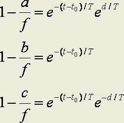
Eliminate the common exponential term.
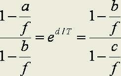
Eliminate the remaining exponential term by setting the fractions equal.
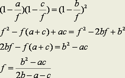
And solve for f. The final closed form solution has three multiplications, three subtractions, and one division, a much lower computational load for the control processor. One multiplication can be eliminated as shown in in the code sample.
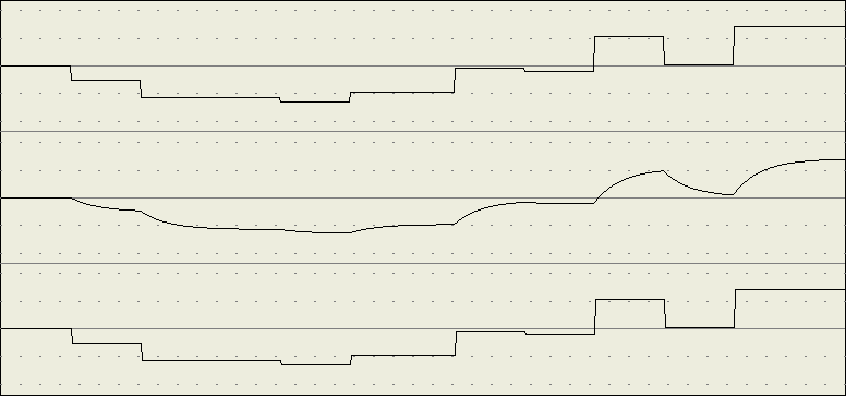
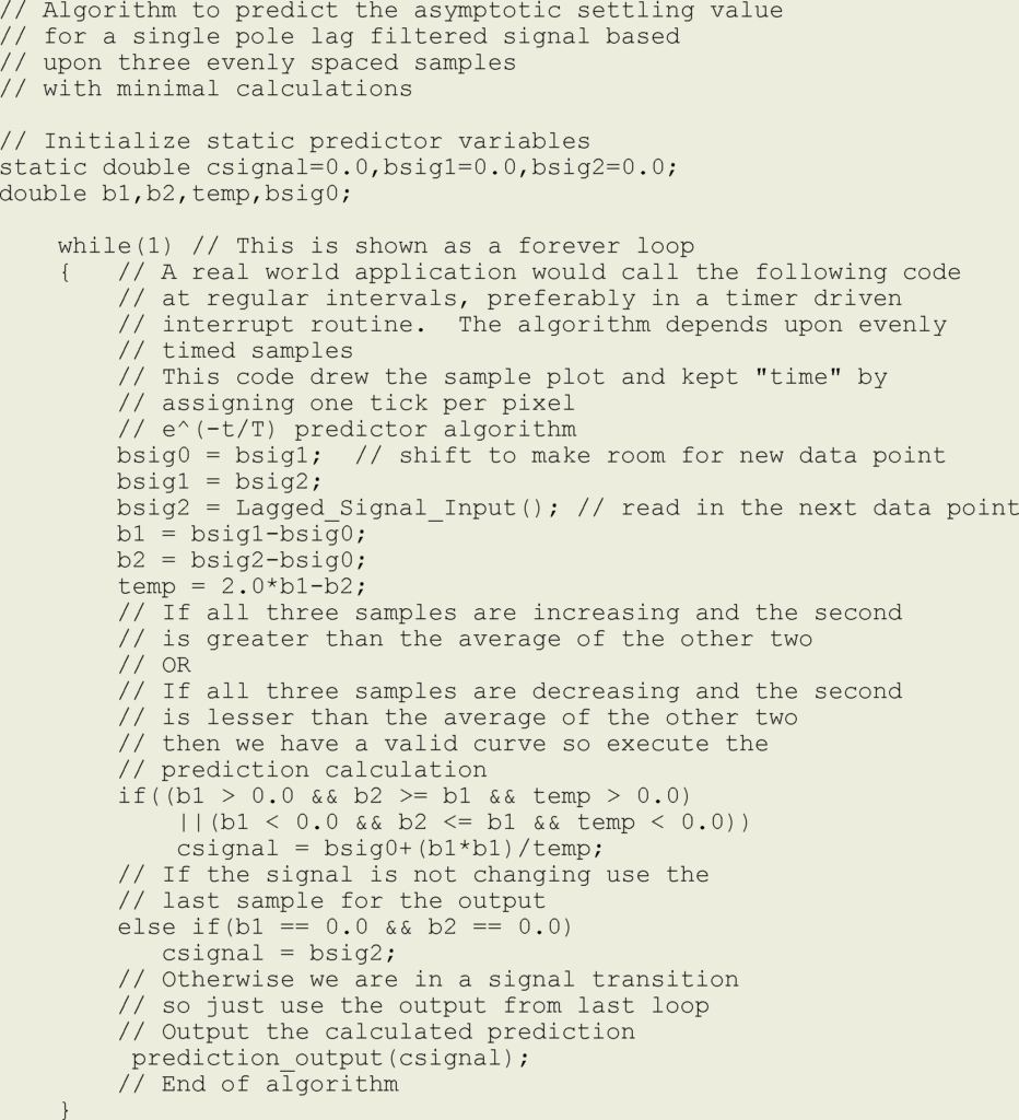
Lag final value predictor performance. 1: Random input, 2: lag response, 3: Algorithm below run on the second line data in real time.
In the actual application the lag data is constantly sampled and processed. Each new sample takes the place of the oldest of three and the predicted value is recalculated allowing real time tracking as shown above. This algorithm was developed for a control system that needed to predict the final settling value of a temperature probe in a hot air stream. The thermal lag of the probe element inside its protective thermowell made the response much to slow to accurately keep the process temperature within limits.
Please leave any comments in my comments post.