While measuring relay response times I noticed an unusual effect. I was working on a (relatively) high power pulse project using automotive relays. I was trying to maximize the repetition rate while maintaining adequate dwell time to charge the high voltage circuit. Measuring a typical 40 amp automotive relay with a reverse diode across the coil yielded the following delay times.
With diode: turn on: N.O. make – 5.0ms, turn off: N.O. break – 6.7ms.
The diode clamps the inductive spike from the coil by recirculating the current. The problem is with almost no voltage across the coil the current and thus the magnetic field takes a long time to decay. Hence the long break time. A standard remedy is to place a zener diode in series with the catch diode. Using a 12 volt zener with a 12 volt relay yields the following delay times.
With diode and zener: turn on: N.O. make- 5.6ms, turn off: N.O. break – 2.6ms.
A 61% reduction in turn off time. Great. But somehow, the turn on time which should have nothing to do with the diode/zener increased by 12%. Weird. After rechecking everything and some thought and other measurements I figured out what was going on.
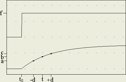
When voltage is applied to the relay coil the inductance of the coil slows the build up of current and the resulting magnetic field. Once the field strength of the core exceeds the strength of the return spring, the armature starts moving. This takes 3.1ms with the diode and 3.7ms with the zener in repetitive mode. Then the armature takes 1.9ms to move to the N.O. contact. When coil voltage is removed the coil inductance tries to keep the current flowing by reversing the voltage.
For the diode version this reverse voltage is clamped t 0.6 volts which lets the coil current slowly decrease for 6.7ms when the field is low enough to release the armature which returns to rest under spring tension in another 1.5ms.
For the zener+diode version the reverse voltage is clamped at 12.6 volts which absorbs the coil energy much much more quickly. The coil inductance holds this voltage for 3.2ms and then decays for a few ms. The current has been decaying continuously and allows the N.O. contact to open after 2.6ms.
The turn on anomaly is due to the parasitic coil capacitance and the relay core hysteresis. With the simple diode circuit the coil is never exposed to reverse polarity current so the magnetic core simply tracks back and forth on the same side of its hysteresis curve. With the zener circuit, after the coil current decays to zero, the 12.6 volt reverse polarity across the coil has charged up the parasitic capacitance of the coil. This now discharges in a reverse current through the coil. This can be observed as the slow decay of the coil voltage from the 12.6 volt peak. This reverse polarity current moves the the iron core of the relay to the other side of its hysteresis curve. The next time the relay coil is energized the coil current has to ramp up enough to demagnetize the reversed core and remagnetize it in the forward direction before the armature can start to move. This causes the additional 0.6ms turn on delay.
The spambots are getting out of hand : Please leave comments, friend, using the post in my comments category. 🙂